Lucas-Kanade Image Alignment
We highly recommend that you render all matplotlib figures inline the Jupyter notebook for the best menpowidgets experience. This can be done by running
%matplotlib inline1. Definition
The aim of image alignment is to find the location of a constant template in an input image . Note that both and are vectorized. This alignment is done by estimating the optimal parameters values of a parametric motion model. The motion model consists of a Warp function which maps each point within a target (reference) shape to its corresponding location in a shape instance. The identity warp is defined as . The warp function in this case is driven by an affine transform, thus consists of 6 parameters.
The Lucas-Kanade (LK) optimization problem is expressed as minimizing the norm with respect to the motion model parameters . Let's load an image and create a template from it
import menpo.io as mio
takeo = mio.import_builtin_asset.takeo_ppm()
# Use a bounding box of ground truth landmarks to create template
takeo.landmarks['bounding_box'] = takeo.landmarks['PTS'].lms.bounding_box()
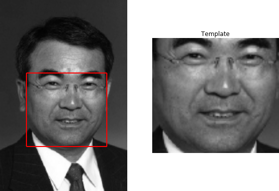
template = takeo.crop_to_landmarks(group='bounding_box')
The image and template can be visualized as:
%matplotlib inline
import matplotlib.pyplot as plt
plt.subplot(121)
takeo.view_landmarks(group='bounding_box', line_colour='r', line_width=2,
                     render_markers=False)
plt.subplot(122)
template.view()
plt.gca().set_title('Template');
2. Optimization and Residuals
The existing gradient descent optimization techniques [1] are categorized as: (1) forward or inverse depending on the direction of the motion parameters estimation and (2) additive or compositional depending on the way the motion parameters are updated.
Forward-Additive
Lucas and Kanade proposed the FA gradient descent in [2]. By using an additive iterative update of the parameters, i.e. , and having an initial estimate of , the cost function is expressed as minimizing with respect to . The solution is given by first linearizing around , thus using first order Taylor series expansion at . This gives , where is the image Jacobian, consisting of the image gradient evaluated at and the warp jacobian evaluated at . The final solution is given by where is the Gauss-Newton approximation of the Hessian matrix. This method is forward because the warp projects into the image coordinate frame and additive because the iterative update of the motion parameters is computed by estimating a incremental offset from the current parameters.
Forward-Compositional
Compared to FA, in FC gradient descent we have the same warp direction for computing the parameters, but a compositional update of the form . The minimization cost function in this case takes the form and the linearization is , where the composition with the identity warp is . The image Jacobian in this case is expressed as . Thus, with this formulation, the warp Jacobian is constant and can be precomputed, because it is evaluated at . This precomputation slightly improves the algorithm's computational complexity compared to the FA case, even though the compositional update is more expensive than the additive one.
Inverse-Compositional
In the IC optimization, the direction of the warp is reversed compared to the two previous techniques and the incremental warp is computed with respect to the template [1, 3]. The goal in this case is to minimize with respect to . The incremental warp is computed with respect to the template , but the current warp is still applied on the input image. By linearizing around and using the identity warp, we have where . Consequently, similar to the FC case, the increment is where the Hessian matrix is . The compositional motion parameters update in each iteration is . Since the gradient is always taken at the template, the warp Jacobian and thus the Hessian matrix inverse remain constant and can be precomputed. This makes the IC algorithm both fast and efficient.
Residuals and Features
Apart from the Sum of Squared Differences (SSD) residual presented above, menpofit includes implementations for
SSD on Fourier domain [4], Enhanced Correlation Coefficient (ECC) [5], Image Gradient [6] and Gradient Correlation [6] residuals.
Additionally, all LK implementations can be applied using any kind of features. For a study on the effect of various feature functions on the LK image alignement, please
refere to [7].
Example
In menpofit, an LK Fitter object with Inverse-Compositional optimization can be obtained as:
from menpofit.lk import LucasKanadeFitter, InverseCompositional, SSD
from menpo.feature import no_op

fitter = LucasKanadeFitter(template, group='bounding_box',
                           algorithm_cls=InverseCompositional, residual_cls=SSD,
                           scales=(0.5, 1.0), holistic_features=no_op)
where we can define different types of features and scales. Remember that most objects can print information about themselves:
print(fitter)
which returns
Lucas-Kanade Inverse Compositional Algorithm
 - Sum of Squared Differences Residual
 - Images warped with DifferentiableAlignmentAffine transform
 - Images scaled to diagonal: 128.35
 - Scales: [0.5, 1.0]
   - Scale 0.5
     - Holistic feature: no_op
     - Template shape: (44, 48)
   - Scale 1.0
     - Holistic feature: no_op
     - Template shape: (87, 96)
3. Alignment and Visualization
Fitting a LucasKanadeFitter to an image is as simple as calling its fit_from_bb method.
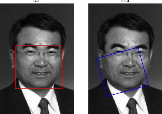
We will attempt to fit the cropped template we created earlier onto a perturbed version of the original image, by adding
noise to its ground truth bounding box. Note that noise_percentage is too large in order to create a very challenging initialization.
from menpofit.fitter import noisy_shape_from_bounding_box

gt_bb = takeo.landmarks['bounding_box'].lms
# generate perturbed bounding box
init_bb = noisy_shape_from_bounding_box(fitter.reference_shape, gt_bb,
                                        noise_percentage=0.1,
                                        allow_alignment_rotation=True)
# fit image
result = fitter.fit_from_bb(takeo, init_bb, gt_shape=gt_bb, max_iters=80)
The initial and final bounding boxes can be viewed as:
result.view(render_initial_shape=True)
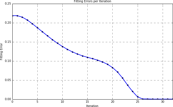
and the alignment error per iteration as:
result.plot_errors()
Of course, the fitting result can also be viewed using a widget:
result.view_widget()
Finally, by using the following code
from menpowidgets import visualize_images
visualize_images(fitter.warped_images(result.image, result.shapes))
we can visualize the warped image per iteration as:
4. References
[1] S. Baker, and I. Matthews. "Lucas-Kanade 20 years on: A unifying framework", International Journal of Computer Vision, vol. 56, no. 3, pp. 221-255, 2004.
[2] B.D. Lucas, and T. Kanade, "An iterative image registration technique with an application to stereo vision", International Joint Conference on Artificial Intelligence, 1981.
[3] S. Baker, and I. Matthews. "Equivalence and efficiency of image alignment algorithms", IEEE Conference on Computer Vision and Pattern Recognition, 2001.
[4] A.B. Ashraf, S. Lucey, and T. Chen. "Fast Image Alignment in the Fourier Domain", IEEE Conference on Computer Vision and Pattern Recognition, 2010.
[5] G.D. Evangelidis, and E.Z. Psarakis. "Parametric Image Alignment Using Enhanced Correlation Coefficient Maximization", IEEE Transactions on Pattern Analysis and Machine Intelligence, vol. 30, no. 10, pp. 1858-1865, 2008.
[6] G. Tzimiropoulos, S. Zafeiriou, and M. Pantic. "Robust and Efficient Parametric Face Alignment", IEEE International Conference on Computer Vision, 2011.
[7] E. Antonakos, J. Alabort-i-Medina, G. Tzimiropoulos, and S. Zafeiriou. "Feature-based Lucas-Kanade and Active Appearance Models", IEEE Transactions on Image Processing, vol. 24, no. 9, pp. 2617-2632, 2015.