Point Distribution Model
- Definition
- Active components
- Generating new instances
- Visualization
- Projection and reconstruction
- API Documentation
We highly recommend that you render all matplotlib figures inline the Jupyter notebook for the best menpowidgets experience. This can be done by running
%matplotlib inline1. Definition
A Point Distribution Model (PDM) is a statistical parametric model of the shape of the deformable obect, which is an essential part for many state-of-the-art deformable models.
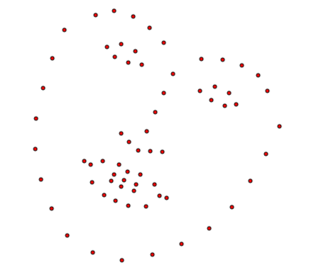
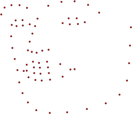
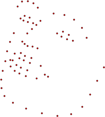
Let us denote a shape instance of an object with landmark points as a vector which consists of the Cartesian coordinates of the points . Assume that we have a set of training shapes . For this demonstration, we will load all the shapes of LFPW trainset:
from pathlib import Path
import menpo.io as mio
from menpo.visualize import print_progress

path_to_lfpw = Path('/path/to/lfpw/trainset/')

training_shapes = []
for lg in print_progress(mio.import_landmark_files(path_to_lfpw / '*.pts', verbose=True)):
    training_shapes.append(lg['all'])
and visualize them as:
%matplotlib inline
from menpowidgets import visualize_pointclouds
visualize_pointclouds(training_shapes)
The construction of a PDM commonly involves the following steps:
- Align the set of training shapes using Generalized Procrustes Analysis, which will remove the similarity transform components (scaling, in-plane rotation, translation) from the shapes.
- Apply Principal Component Analysis (PCA) on the aligned shapes. This involves first centering the aligned shapes by subtracting the mean shape and then computing the basis of eigenvectors .
- Further augment the acquired subspace with four eigenvectors that control the global similarity transform of the object, re-orthonormalize [1] and keep the first eigenvectors. This results to a linear shape model of the form where is an orthonormal basis of eigenvectors and is the mean shape vector.
The above procedure can be very easily performed using menpofit's OrthoPDM class as:
from menpofit.modelinstance import OrthoPDM
shape_model = OrthoPDM(training_shapes, max_n_components=None)
Information about the PCA model that exists in the PDM can be retrieved as:
print(shape_model)
which prints:
Point Distribution Model with Similarity Transform
 - total # components:      136
 - # similarity components: 4
 - # PCA components:        132
 - # active components:     4 + 132 = 136
 - centred:                 True
 - # features:              136
 - kept variance:           7.6e+03  100.0%
 - noise variance:          0.025  0.0%
 - components shape:        (132, 136)
2. Active Components
Note that in the previous printing message all the available components are active. This means that when using the model for any kind of operations such as projection or reconstruction, then the whole subspace will be used. Normally, you need to use less components in order to remove the noise that is captured by the last components. This can be done by setting the number of active components either by explicitly defining the desired number as
shape_model.n_active_components = 20
or by providing the percentage of variance to be kept as
shape_model.n_active_components = 0.95
Let's print again the OrthoPDM object
print(shape_model)
which would now return
Point Distribution Model with Similarity Transform
 - total # components:      136
 - # similarity components: 4
 - # PCA components:        132
 - # active components:     4 + 16 = 20
 - centred:                 True
 - # features:              136
 - kept variance:           7.3e+03  95.2%
 - noise variance:          3.1  0.0%
 - components shape:        (16, 136)
3. Generating New Instances
A new shape instance can be generated as where is the shape parameters vector.
You can generate a new shape instance using only the similarity model (which will naturally apply a similarity transform on the mean shape) as
instance = shape_model.similarity_model.instance([100., -300., 0., 0.])
instance.view(render_axes=False);
Similarly, a new instance using only the PCA components can be generated as
instance = shape_model.model.instance([2., -2., 2., 1.5], normalized_weights=True)
instance.view(render_axes=False);
Note that in this case, the weights that are provided are normalized with respect to the corresponding eigenvalues.
A combined instance using all the components can be generated by using the from_vector_inplace() method as
params = [100., -300., 0., 0., 140., -100., 15., 5.]
shape_model.from_vector(params).target.view(render_axes=False);
which returns the following instance
4. Visualization
The PCA components of the OrthoPDM can be explored using an interactive widget as:
from menpowidgets import visualize_shape_model
visualize_shape_model(shape_model.model)
5. Projection and Reconstruction
A shape instance can be theoretically projected into a given shape model as Similarly, the reconstruction of a shape instance is done as:
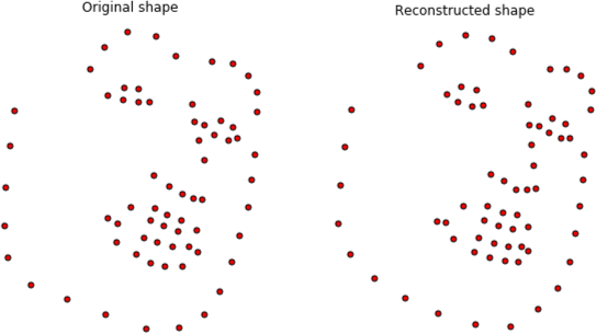
OrthoPDM makes it very easy to reconstruct a shape isntance by setting its target.
Let's load Einstein's shape, reconstruct it
using the active components (similarity and PCA) and visualize the result:
import matplotlib.pyplot as plt

# Import shape and reconstruct
shape = mio.import_builtin_asset.einstein_pts().lms
shape_model.set_target(shape)

# Visualize
plt.subplot(121)
shape.view(render_axes=False, axes_x_limits=0.05, axes_y_limits=0.05)
plt.gca().set_title('Original shape')
plt.subplot(122)
shape_model.target.view(render_axes=False, axes_x_limits=0.05, axes_y_limits=0.05)
plt.gca().set_title('Reconstructed shape');
The procedure that is applied inside set_target() involves the following steps:
import matplotlib.pyplot as plt
from menpo.transform import AlignmentAffine

# Import shape
shape = mio.import_builtin_asset.einstein_pts().lms

# Find the affine transform that normalizes the shape
# with respect to the mean shape
transform = AlignmentAffine(shape, shape_model.model.mean())

# Normalize shape and project it
normalized_shape = transform.apply(shape)
weights = shape_model.model.project(normalized_shape)
print("Weights: {}".format(weights))

# Reconstruct the normalized shape
reconstructed_normalized_shape = shape_model.model.instance(weights)

# Apply the pseudoinverse of the affine tansform
reconstructed_shape = transform.pseudoinverse().apply(reconstructed_normalized_shape)

# Visualize
plt.subplot(121)
shape.view(render_axes=False, axes_x_limits=0.05, axes_y_limits=0.05)
plt.gca().set_title('Original shape')
plt.subplot(122)
reconstructed_shape.view(render_axes=False, axes_x_limits=0.05, axes_y_limits=0.05)
plt.gca().set_title('Reconstructed shape');